Jupyter
Contents
JupyterLab (Web) Tutorial - KENET HPC Cluster
Overview
JupyterLab is an interactive web-based environment for notebooks, code, and data. It provides an ideal platform for data science, scientific computing, and machine learning workflows, allowing researchers to combine code execution, rich text, visualizations, and interactive outputs in a single document.
Use Cases: JupyterLab is particularly well-suited for interactive data analysis and visualization, machine learning model development and experimentation, creating reproducible research notebooks, teaching and sharing computational narratives, and real-time data exploration with optional GPU acceleration.
Access: JupyterLab is available through the KENET Open OnDemand web portal at https://ondemand.vlab.ac.ke
Code Examples: All code examples for this tutorial are available in our GitHub repository at https://github.com/Materials-Modelling-Group/training-examples
Prerequisites
Before using JupyterLab, you should have an active KENET HPC cluster account with access to the Open OnDemand portal. Basic knowledge of Python, R, or Julia will be helpful, and you should have your data files stored in your home directory at /home/username/localscratch.
Launching JupyterLab
Step 1: Access Interactive Apps
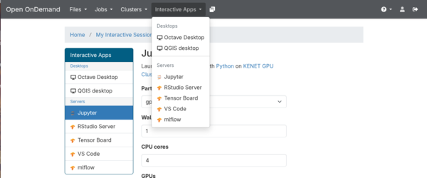
Begin by logging into Open OnDemand at https://ondemand.vlab.ac.ke using your KENET credentials. Once logged in, click the Interactive Apps menu in the top navigation bar, then select JupyterLab from the dropdown list of available applications.
Step 2: Configure Job Parameters
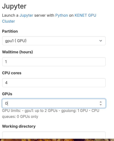
The job submission form allows you to specify the computational resources needed for your JupyterLab session. Fill in the form according to your workload requirements using the table below as a guide.
| Parameter | Description | Recommended Value |
|---|---|---|
| Partition | Queue for job execution | normal (CPU) or gpu (GPU tasks)
|
| Walltime | Maximum runtime in hours | 2 hours for testing, up to 192 for long jobs
|
| CPU Cores | Number of processor cores | 4-8 cores (adjust based on workload)
|
| Memory | RAM allocation | 16 GB for data science, 32 GB for large datasets
|
| Working Directory | Starting directory | /home/username or your project folder
|
Tip: For GPU-accelerated deep learning tasks, select the gpu partition and specify the number of GPUs needed for your work.
Step 3: Submit and Wait
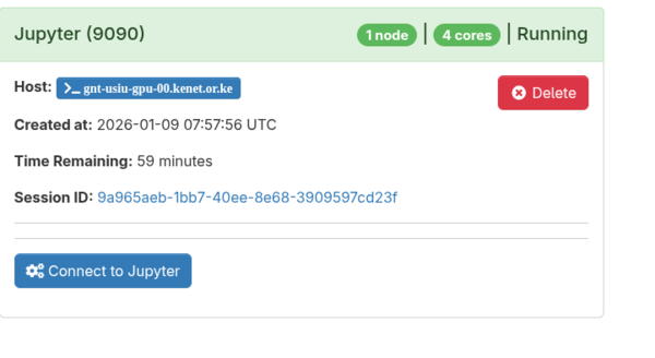
After configuring your job parameters, click the Launch button to submit your job to the cluster scheduler. The job will initially show a "Queued" status while waiting for resources to become available. Once resources are allocated (typically within 30-60 seconds), the status will change to "Running" and a Connect to JupyterLab button will appear. Click this button to open your JupyterLab session in a new browser tab.
Quick Start Guide
Creating Your First Notebook
When JupyterLab opens, you will see the Launcher interface. To create a new notebook, click File → New → Notebook from the menu, or simply click the Python 3 tile in the Launcher. You will be prompted to select a kernel, which determines the programming language and environment for your notebook. Choose Python 3, R, or Julia depending on your needs.
Basic Cell Operations
Notebooks consist of cells where you can write and execute code. To see a basic example of creating a simple plot, refer to the 01_basic_plotting.py example in our GitHub repository. Press Shift+Enter to run any cell and see the output immediately below it.
There are three main cell types in JupyterLab. Code cells contain executable code and are the default type. Markdown cells contain formatted text, equations, and documentation. Raw cells contain plain text that is not executed or formatted.
Installing Python Packages
You can install additional Python packages directly from within a notebook cell using pip. The proper syntax is shown in the 00_package_installation.sh file in our GitHub repository. Always use the --user flag to install packages in your personal home directory rather than attempting system-wide installation, which will fail due to permissions.
Important: After installing new packages, you must restart the kernel by selecting Kernel → Restart from the menu for the packages to be recognized.
Common Tasks
Task 1: Loading Data from Cluster Storage
Loading data from files stored on the cluster is straightforward using pandas or other data libraries. You can read data from your home directory or from the faster scratch storage. See the example in 02_loading_data.py in our GitHub repository for the complete code showing how to read CSV files from both locations.
Task 2: Using GPU for Deep Learning
If you launched your session on the GPU partition, you can leverage GPU acceleration for deep learning tasks. TensorFlow and PyTorch will automatically detect and use available GPUs. The 03_gpu_tensorflow.py example demonstrates how to check GPU availability and create a simple neural network model that will automatically utilize GPU resources when available.
Task 3: Parallel Processing with Dask
For large datasets that don't fit in memory, Dask provides parallel processing capabilities that work seamlessly with pandas syntax. The 04_dask_parallel.py example shows how to read large datasets using Dask and perform grouped aggregations efficiently across multiple cores.
Task 4: Creating Interactive Visualizations
Plotly provides interactive visualizations that work well in JupyterLab, allowing you to zoom, pan, and explore your data dynamically. See 05_plotly_interactive.py for an example of creating an interactive scatter plot with categorical coloring.
Tips & Best Practices
Performance Optimization
When working with computationally intensive tasks, request the GPU partition for deep learning work. For parallel data processing, allocate 4-8 cores to take advantage of multi-core operations. Store large datasets in /scratch/username/ rather than your home directory for significantly faster I/O performance. You can profile cell execution time using the double-percent time magic command at the beginning of a cell. Remember to close notebooks when you are finished to free up memory for other tasks.
Session Management
Notebooks are automatically saved every 120 seconds, so your work is protected from unexpected disconnections. However, be aware that the kernel continues running even if you close the browser tab. If you encounter memory issues, restart the kernel by selecting Kernel → Restart from the menu. Variables and data persist between cells until you restart the kernel, so you can build up your analysis incrementally across multiple cells.
Security Best Practices
Never hardcode passwords or API keys directly in your notebooks. Instead, use environment variables which you can access with the os.getenv function. Before sharing notebooks with colleagues, clear any sensitive outputs by selecting Cell → All Output → Clear from the menu. This ensures that confidential data or credentials are not inadvertently shared.
Example Workflows
Example 1: Data Science Pipeline
Objective: This workflow demonstrates how to load, clean, analyze, and visualize research data in a reproducible manner.
Begin by launching JupyterLab with 8 cores and a 6-hour walltime to ensure adequate resources for your analysis. Create a new notebook named analysis.ipynb and follow the steps in the workflows/01_data_science_pipeline.py example from our GitHub repository.
The workflow starts by loading your data, then explores the data structure and summary statistics to understand data types, missing values, and basic distributions. Next, clean the data by handling missing values appropriately and identifying and addressing any outliers. Use seaborn or matplotlib to create visualizations that reveal patterns and relationships in your data. Export your cleaned data for use in subsequent analyses, and download your notebook by right-clicking on it in the file browser and selecting Download.
Example 2: Machine Learning Experiment
Objective: Train and compare multiple machine learning models to identify the best performing approach for your dataset.
Launch JupyterLab with the GPU partition if you plan to use deep learning models. Follow the complete workflow in workflows/02_ml_experiment.py which demonstrates how to load data, split it into training and testing sets, train multiple model types, compare their performance, and save the best performing model for later use.
Example 3: Geospatial Analysis
Objective: Process and visualize geographic data using specialized geospatial libraries.
The workflows/03_geospatial_analysis.py example walks through installing geospatial packages, loading shapefile or GeoJSON data, performing spatial operations such as buffering or intersection, and creating an interactive map using folium. The final map can be exported to HTML for easy sharing and presentation.
Keyboard Shortcuts
Mastering keyboard shortcuts will significantly improve your productivity in JupyterLab. Press Shift + Enter to run the current cell and move to the next one. In command mode (press Escape to enter), press B to insert a new cell below the current cell, or A to insert one above. Delete a cell by pressing D twice in quick succession. Convert a cell to Markdown by pressing M, or back to Code by pressing Y. Save your notebook with Ctrl + S. Access the command palette with Ctrl + Shift + C to search for any command. Comment or uncomment code with Ctrl + /. Undo the last cell operation by pressing Z in command mode.
Troubleshooting
Problem: Session won't start or stays in "Queued" state
This typically occurs when no computational resources are available or the queue is full. Try reducing the number of requested cores or memory in your job parameters. Switch to a different partition such as debug for quick testing with limited resources. Check the cluster status on the dashboard to see current load. If the problem persists after trying these solutions, contact KENET support for assistance.
Problem: Kernel dies or becomes unresponsive
A dying or unresponsive kernel usually indicates an out-of-memory condition or that your code has entered an infinite loop. Restart the kernel by selecting Kernel → Restart from the menu. Clear all outputs by selecting Edit → Clear All Outputs to free up memory. For testing, reduce the size of your data or use sampling to work with a subset. In your next session, request more memory to accommodate your full dataset.
Problem: "Module not found" error
This error appears when a required Python package is not installed in your environment. Refer to the 00_package_installation.sh example in our GitHub repository for the correct installation syntax. After installation, you must restart the kernel for the new package to be recognized.
Problem: Can't save notebook
Inability to save usually results from exceeding your disk quota or a permissions issue. Check your disk usage from a terminal or notebook cell. Delete unnecessary files or move large files to scratch storage. Verify file permissions to ensure you have write access to the directory.
Problem: GPU not detected
If your code cannot detect the GPU, first verify that you selected the GPU partition when launching your JupyterLab session. The 03_gpu_tensorflow.py example includes code to check GPU availability. If no GPUs are detected, you will need to end your current session and relaunch with the GPU partition selected.
Additional Resources
The official JupyterLab documentation is available at https://jupyterlab.readthedocs.io/ and provides comprehensive information about all features. For Jupyter Notebook basics, see https://jupyter-notebook.readthedocs.io/. KENET HPC usage guidelines are documented at https://training.kenet.or.ke/index.php/HPC_Usage.
For learning JupyterLab, DataCamp provides an excellent tutorial at https://www.datacamp.com/tutorial/tutorial-jupyter-notebook, and Real Python offers a comprehensive introduction at https://realpython.com/jupyter-notebook-introduction/.
Key Python libraries for data science include Pandas for data manipulation (https://pandas.pydata.org/), NumPy for numerical computing (https://numpy.org/), Matplotlib for plotting (https://matplotlib.org/), and Scikit-learn for machine learning (https://scikit-learn.org/).
Code Examples Repository: All code examples referenced in this tutorial are available at https://github.com/Materials-Modelling-Group/training-examples.git
For support, contact KENET at support@kenet.or.ke, consult the documentation at https://training.kenet.or.ke/index.php/HPC_Usage, or access the Open OnDemand portal at https://ondemand.vlab.ac.ke.
Version Information
This tutorial documents JupyterLab version 4.x running Python 3.9 or later. The JupyterLab installation is located at /opt/ohpc/pub/codes/ood/jupyterlab on the cluster. This tutorial was last updated on 2026-01-09 and is currently at version 1.0.
Feedback
If you encounter issues or have suggestions for improving this tutorial, please contact KENET support or submit feedback through the Open OnDemand interface using the feedback button.


