Difference between revisions of "Thematic Examples"

Revision as of 10:30, 9 May 2025

Thematic Examples From Computer Science, Engineering and Computational Modeling and Material Science

We will work through examples based on the following codes:

1. Quantum Espresso (CMMS)
2. YAMBO (CMMS)
3. GROMACS (CMMS)
4. Tensorflow (CS)
5. PyTorch (CS)
6. FluidX3D (Engineering)

CMMS Thematic Area

Gromacs Tutorial

Quantum Espresso Tutorial

Computing The Bandstructure of Silicon

In this tutorial, we will calculate the band structure of bulk Silicon. Silicon is a semi-conductor with a small gap. The calculation will proceed through three broad steps, starting from the self consistent calculation, the non-self consistent calculation, the bands calculation, and finally the post processing. The files required for this exercise can be retreived as follows:

$ cd ~/localscratch/
$ mkdir examples
$ cd examples/
$ git clone https://github.com/Materials-Modelling-Group/training-examples.git
$ cd training-examples/
$ ls 
si.band.david.in  si.nscf.david.in  si.plotbands.in  si.scf.david.in 

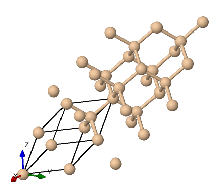
We can visualize the structure using tools like VESTA or Xcrysden, using the input file that specifies the structure si.scf.david.in . This can be done on your computer once you install Xcrysden and copy the input to your device as such:

$ xcrysden --pwi si.scf.david.in 

Which gives us this structure visualization:

Showing the typical diamond like tetrahedral structure. We now call Quantum Espresso and run the three steps, this can be performed in one job for simple short calculations, for longer calculations the three steps can be separated into three jobs. Let us create the three submission scripts.

#!/bin/bash
#SBATCH --job-name=si_scf_normal
#SBATCH --partition=gpu1
#SBATCH --gpus=1
#SBATCH --ntasks-per-node=1
#SBATCH --time=00:10:00
#SBATCH --output=si_scf_%j.out 
#SBATCH --error=si_scf_%j.err

##Load necessary modules
module load applications/gpu/qespresso/7.3.1 

##Set environment variables for QE
cd $HOME/localscratch/examples/training-examples 

##Run QE with GPU support
mpirun -np 1  pw.x -in si.scf.david.in > scf.out

put this in a file named 1scf.job and we submit the same:

$ sbatch 1scf.job

Once this has run, we will have some generated outputs, including wavefunctions and the text file scf.out. Next we prepare the submission script for the nscf step,

#!/bin/bash
#SBATCH --job-name=si_nscf_normal
#SBATCH --partition=gpu1
#SBATCH --gpus=1
#SBATCH --ntasks-per-node=1
#SBATCH --time=00:10:00
#SBATCH --output=si_scf_%j.out 
#SBATCH --error=si_scf_%j.err

##Load necessary modules
module load applications/gpu/qespresso/7.3.1 

##Set environment variables for QE
cd $HOME/localscratch/examples/training-examples 

##Run QE with GPU support
mpirun -np 1  pw.x -in si.nscf.david.in > nscf.out

put this in a file named 2nscf.job and we submit the same:

$ sbatch 2nscf.job

Once this nscf step is done, we now compute the band structure, create the submission script for the bands calculation:

#!/bin/bash
#SBATCH --job-name=si_bands_normal
#SBATCH --partition=gpu1
#SBATCH --gpus=1
#SBATCH --ntasks-per-node=1
#SBATCH --time=00:10:00
#SBATCH --output=si_scf_%j.out 
#SBATCH --error=si_scf_%j.err

##Load necessary modules
module load applications/gpu/qespresso/7.3.1 

##Set environment variables for QE
cd $HOME/localscratch/examples/training-examples 

##Run QE with GPU support
mpirun -np 1 bands -in si.bands.in  > si.bands.out

We have the bulk of the computational work done, we now are left with a post processing steps to obtain results, we now use the plotbands executable for this step:

#!/bin/bash
#SBATCH --job-name=si_ppbands_normal
#SBATCH --partition=gpu1
#SBATCH --gpus=1
#SBATCH --ntasks-per-node=1
#SBATCH --time=00:10:00
#SBATCH --output=si_scf_%j.out 
#SBATCH --error=si_scf_%j.err

##Load necessary modules
module load applications/gpu/qespresso/7.3.1 

##Set environment variables for QE
cd $HOME/localscratch/examples/training-examples 

##Run QE with GPU support
mpirun -np 1 plotband.x  < si.plotband.in

This will produce some new visualization data and a postscript plot, si_bands.ps which should yield an image like this:

CS Thematic Area

TODO

Conda Usage on the cluster

TODO

PyTorch Tutorial

TODO

TensorFlow Tutorial

Engineering Thematic Area

TODO.

FluidX3D Tutorial

TODO

Up: HPC_Usage