Thematic Examples

Thematic Examples From Computer Science, Engineering and Computational Modeling and Material Science

We will work through examples based on the following codes:

1. Quantum Espresso (CMMS)
2. PyTorch (CS)
3. FluidX3D (Engineering)

CMMS Thematic Area

Quantum Espresso Tutorial

Computing The Bandstructure of Silicon

In this tutorial, we will calculate the band structure of bulk Silicon. Silicon is a semi-conductor with a small gap. The calculation will proceed through three broad steps, starting from the self consistent calculation, the non-self consistent calculation, the bands calculation, and finally the post processing. The files required for this exercise can be retreived as follows:

$ cd ~/localscratch/
$ mkdir examples
$ cd examples/
$ git clone https://github.com/Materials-Modelling-Group/training-examples.git
$ cd training-examples/
$ ls 
si.band.david.in  si.nscf.david.in  si.plotbands.in  si.scf.david.in 

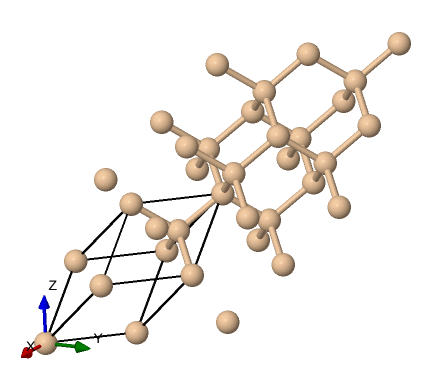
We can visualize the structure using tools like VESTA or Xcrysden, using the input file that specifies the structure si.scf.david.in . This can be done on your computer once you install Xcrysden and copy the input to your device as such:

$ xcrysden --pwi si.scf.david.in 

Which gives us this structure visualization:

Showing the typical diamond like tetrahedral structure. We now call Quantum Espresso and run the three steps, this can be performed in one job for simple short calculations, for longer calculations the three steps can be separated into three jobs. Let us create the appropriate submission scripts. This is a simple seof calculations, but we have split it into multiple jobs for the sake of generality.

#!/bin/bash
#SBATCH --job-name=si_scf_normal
#SBATCH --partition=gpu1
#SBATCH --gpus=1
#SBATCH --ntasks-per-node=1
#SBATCH --time=00:10:00
#SBATCH --output=si_scf_%j.out 
#SBATCH --error=si_scf_%j.err

##Load necessary modules
module load applications/gpu/qespresso/7.3.1 

##Set environment variables for QE
cd $HOME/localscratch/examples/training-examples 

##Run QE with GPU support
mpirun -np 1  pw.x -in si.scf.david.in > scf.out

put this in a file named 1scf.job and we submit the same:

$ sbatch 1scf.job

Once this has run, we will have some generated outputs, including wavefunctions and the text file scf.out. Next we prepare the submission script for the nscf step,

#!/bin/bash
#SBATCH --job-name=si_nscf_normal
#SBATCH --partition=gpu1
#SBATCH --gpus=1
#SBATCH --ntasks-per-node=1
#SBATCH --time=00:10:00
#SBATCH --output=si_scf_%j.out 
#SBATCH --error=si_scf_%j.err

##Load necessary modules
module load applications/gpu/qespresso/7.3.1 

##Set environment variables for QE
cd $HOME/localscratch/examples/training-examples 

##Run QE with GPU support
mpirun -np 1  pw.x -in si.nscf.david.in > nscf.out

put this in a file named 2nscf.job and we submit the same:

$ sbatch 2nscf.job

Once this nscf step is done, we now compute the band structure, create the submission script for the bands calculation:

#!/bin/bash
#SBATCH --job-name=si_bands_normal
#SBATCH --partition=gpu1
#SBATCH --gpus=1
#SBATCH --ntasks-per-node=1
#SBATCH --time=00:10:00
#SBATCH --output=si_scf_%j.out 
#SBATCH --error=si_scf_%j.err

##Load necessary modules
module load applications/gpu/qespresso/7.3.1 

##Set environment variables for QE
cd $HOME/localscratch/examples/training-examples 

##Run QE with GPU support
mpirun -np 1 bands.x -in si.bands.in  > si.bands.out

We have the bulk of the computational work done, we now are left with a post processing steps to obtain results, we now use the plotbands executable for this step:

#!/bin/bash
#SBATCH --job-name=si_ppbands_normal
#SBATCH --partition=gpu1
#SBATCH --gpus=1
#SBATCH --ntasks-per-node=1
#SBATCH --time=00:10:00
#SBATCH --output=si_scf_%j.out 
#SBATCH --error=si_scf_%j.err

##Load necessary modules
module load applications/gpu/qespresso/7.3.1 

##Set environment variables for QE
cd $HOME/localscratch/examples/training-examples 

##Run QE with GPU support

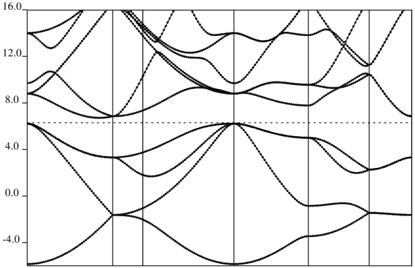
plotband.x < si.plotband.in This will produce some new visualization data and a postscript plot, si_bands.ps which should yield an image like this:

CS Thematic Area

Conda Usage on the cluster

Conda is a python based package manager and (python) environment management tool, used to install and manage multiple versions of software packages and tools. Its typical for it to be installed in a single user's account, and active from the moment a user logs in, however, being that this facility is a cluster, we have opted to provide it to users using our HPC Module system, this should reduce redundancy in the core packages, saving every user from having a local installation in their account. Conda users will have access to all centrally installed packages.

How to activate Conda and View environments

Conda is available in the global list of modules, which can be listed via the module avail command, meaning until you load the module, the conda command is not available.

$ module avail
 --------------------------- /usr/share/modulefiles --------------------
  mpi/openmpi-x86_64
 -------------------- /opt/ohpc/pub/modulefiles --------------------
 applications/gpu/gromacs/2024.4 ...
 ... 
 applications/gpu/python/conda-25.1.1-python-3.9.21
 ...

Let us go a head and load the right module:

$ module load applications/gpu/python/conda-25.1.1-python-3.9.21

We now have the conda command available on the terminal. Let us list the conda environments available by default:

$ conda env list
base                 * /opt/ohpc/pub/conda/instdir
python-3.9.21          /opt/ohpc/pub/conda/instdir/envs/python-3.9.21

And we can load the python-3.9.21 conda environment, this environment provides a set of key ML/AI python frameworks, namely PyTorch and Tensorflow.

$ conda activate python-3.9.21

Tools like Pytorch, TensorFlow and others are available in this environment.

Watch Conda Demo

Object Detection Tutorial (YOLO)

We will take a look at a simple object detection exercise with YOLO. Let us get the files needed for the exercise:

$ cd ~/localscratch/
$ mkdir examples
$ cd examples/
$ git clone https://github.com/Materials-Modelling-Group/training-examples.git
$ cd training-examples/

Now we have to install yolo, and use it to run a simple object detection exercise using the code in the file objdet.py. Place the following in a simple text file 'det.job':

#!/bin/bash
#SBATCH --job-name=si_scf_normal
#SBATCH --partition=gpu1
#SBATCH --gpus=1
#SBATCH --ntasks-per-node=1
#SBATCH --time=00:10:00
#SBATCH --output=si_scf_%j.out 
#SBATCH --error=si_scf_%j.err

##Load necessary modules
module load applications/gpu/python/conda-25.1.1-python-3.9.21
conda activate python-3.9.21
pip install ultralytics

cd $HOME/localscratch/examples/training-examples/
python3  objdet.py

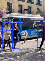
It should produce two images on the disk, the original and the annotated, showing the object detection:

Engineering Thematic Area

FluidX3D Tutorial

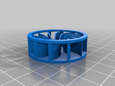
In this tutorial we will compute the airflow around a Fan using and implementation of Lattice Boltzmann CDF in FluidX3D. The geometry to be used will be similar to this Fan: SOLID BOTTOM

FluidX3D is a C++ code with support for GPU acceleration, and requires that we write some code to setup the calculation. Let us retreive the code and data for the calculation:

$ cd ~/localscratch/
$ mkdir cfd
$ cd cfd
$ git clone https://github.com/Materials-Modelling-Group/training-examples.git
$ https://github.com/ProjectPhysX/FluidX3D.git
$ cp training-examples/{setup.cpp,defines.hpp} FluidX3D/src
$ mkdir stl 
$ wget https://cdn.thingiverse.com/assets/1d/89/dd/cb/fd/FAN_Solid_Bottom.stl?ofn=RkFOX1NvbGlkX0JvdHRvbS5zdGw= -O stl/Fan.stl

Once we have the files, we can load the right modules, and compile the example, place the following in a simple file: cfd.job

#!/bin/bash
#SBATCH --job-name=si_scf_normal
#SBATCH --partition=gpu1
#SBATCH --gpus=1
#SBATCH --ntasks-per-node=1
#SBATCH --time=00:10:00
#SBATCH --output=si_scf_%j.out 
#SBATCH --error=si_scf_%j.err

##Load necessary modules
module load devel/nvidia-hpc/24.11

cd $HOME/localscratch/cfd/ 
cd FluidX3D
./make.sh

And submit it to slurm via cfd.job, and let it run. This will generate the outputs in ./bin/export, this was specified in the setup.cpp code instructions. We can now convert these snapshots into a video file using FFMPEG especially compiled with GPU support on the cluster, however, only open codecs like libopenh264 are enabled in this ffmpeg module. Place the following in a simple file named encode.job

#!/bin/bash
#SBATCH --job-name=si_scf_normal
#SBATCH --partition=gpu1
#SBATCH --gpus=1
#SBATCH --ntasks-per-node=1
#SBATCH --time=00:10:00
#SBATCH --output=si_scf_%j.out 
#SBATCH --error=si_scf_%j.err

##Load necessary modules
module load applications/gpu/ffmpeg/git 

cd $HOME/localscratch/cfd/FluidX3D/bin
ffmpeg -y -hwaccel cuda  -framerate 60 -pattern_type glob -i "export/image-*.png" -c:v libopenh264   -pix_fmt yuv420p -b:v 24M "video.mp4"

Submit the job via slurm

$ sbatch encode.job

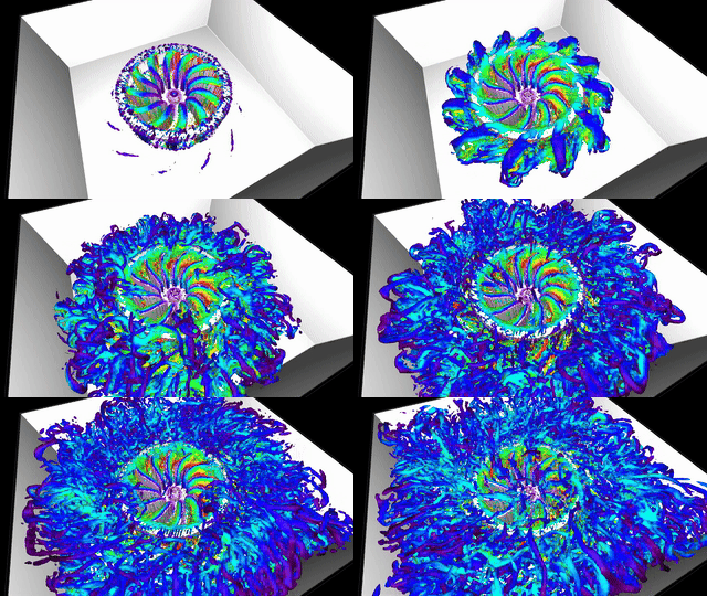
Once complete, it will produce the following video inside the FluidX3D/bin directory:

Watch CFD Demo

Up: HPC_Usage